Response Time Measurement

Introduction

Response time is often considered one of the most important specifications when choosing a new monitor and has been since TFT displays first came to the market. Anyone wanting to use their screen for games or movies, where fast moving scenes are common, will be concerned with how quickly the screen can cope with those changes. How quickly a pixel can respond (its response time) has a huge impact on blurring and ghosting in moving images and it is for those reasons why response time is so regularly discussed. We discuss response times in more detail in our specs section for those who would like more background information.

We have always conducted tests in our reviews to try and give readers an idea of the responsiveness of any given screen, whether its suitable for fast paced action, and how it compares with other displays in the market. This has been based on trying to capture and explain the responsiveness in practice and each review contains tests and analysis based on the use of the now famous PixPerAn tool. We are of course always looking at new ways to improve our testing methodology and in this article we will explain a new process we are introducing to help measure and record response times even more accurately for our readers.

Response Time Specs

There are currently two methods which manufacturers use for measuring and reporting response time for their displays. This is dictated really by whether the screen is using Response Time Compensation (RTC), otherwise known as ‘overdrive’ to improve their pixel response times.

For displays where overdrive is not used, manufacturers will generally quote the more traditional ISO 13406-2 response time which will represent a measurement for the pixels changing from black > white > black (0-255-0). This ISO response time is made up of the rise and fall time as the pixel changes from one state to the other and then back again. You will see specs quoted where the response time is listed on its own, without a “G2G” (grey to grey) after it. Typically there are limits for each panel technology of how far these ISO response times can be pushed. For a TN Film panel, the fastest ISO response time is usually quoted as 5ms. For VA matrices it is ~12ms and for IPS is is ~16ms. On these displays without overdrive the ISO 0-255-0 change is the fastest since the highest voltage is applied to re-orientate the pixels. Manufacturers quote this spec but you need to keep in mind that the other transitions (between different grey shades for example) will be higher and are not specified at all. In fact in normal use it would be quite rare to see a full black > white transition, and changes between different grey scales (i.e. between different colours) are far more common. Unfortunately the spec provided will not tell you how fast these are at all. Keep in mind therefore that the more important grey to grey transitions may be much slower than the quoted ISO response time, and so overall performance in practice may vary significantly. This is particularly noticeable when looking at VA or IPS panels without overdrive, where G2G transitions can be very slow. This ISO response time is only really quoted for screens without overdrive being used, and in today’s market that is fairly rare really.

For displays which do use overdrive, manufacturers go a different route with their specs. Where overdrive is used it will result in a marked improvement in actual perceived responsiveness and overall the more important grey to grey transitions will be greatly sped up. Since the ISO response time is no longer the fastest (since higher voltages are now being applied to other transitions), manufacturers instead quote their best grey to grey (G2G) response time in their spec. While this is still somewhat misleading since its only the best case, it does give you a better view of how the screen might perform in practice as we at least know overdrive is being used in screens where G2G figures are quoted, which should result in an overall faster matrix. For instance a screen with a quoted 4ms G2G response time should perform much better in practice than a 5ms ISO response time screen (without overdrive), despite the spec only suggesting a 1ms difference. The spec being offered is still not ideal but does give you a better indication of the response times to expect.

Our New Testing Methodology

To help give a more honest view of how a panel performs in real life we have developed a new testing method which will feature in our forthcoming reviews. This method has been / is used by other review sites and provides a better understanding of the real-World pixel response times. Our method is very similar to the existing oscilloscope + photosensor methods being used already so hopefully readers will be somewhat familiar with the principles.

To perform the measurement a custom-made photosensor device is attached to the screen and used to track changes in the brightness levels. A special software program is used to simulate the changes between different shades from the full range of 0 (black) to 255 (white). From there, the photosensor measures the brightness change and converts it into a voltage which is passed to an Oscilloscope.

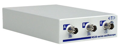
We use an ETC M526 Digital Storage Oscilloscope supplied to us by ETC Ltd, a Slovakian company who specialise in measurement equipment such as this with a very good price to performance ratio.

The Oscilloscope and accompanying software produces oscillograms such as that shown above which allow us to observe and measure the response time of the pixels, and determine how quickly the pixel changes from one state to another. Depending on the scale used on the oscilloscope, the grid lines can be used to calculate the response time.

The graph is interpreted as shown above. The lower flat line is the starting shade and the top line is the final shade being tested. The vertical parts of the green graph signify the response time as the pixel changes from one state to another. The upwards curve is the rise time (i.e. the change from the darker shade to the lighter shade), and the downwards line is the fall time (i.e. the change from lighter to darker shade). The speed of these rise and fall times is part of what we will want to measure and will vary depending on the screen of course, and on the requested transition between different shades of grey. The above graph shows a fairly neat response time oscillogram with a pretty straightforward curve.

What might be more typical though is an oscillogram such as that shown above. You may note that the rise time actually shoots a little above the required level before dropping back down. The fall time does the same thing, dropping a little too far before it levels out at the desired shade. This is a classic case of overshoot caused by a RTC / overdrive impulse. This may vary significantly from one screen to another as well, depending on the level of overdrive impulse being used, how aggressively it is applied and how well the internal electronics are controlling the impulse.

The oscilloscope software allows us to define the lower and upper levels as shown above using the horizontal red and blue lines. These represent the two shades we are switching between.

You can then use the vertical grid lines within the software to mark the interception points where the response time curve crosses the horizontal lines. The software tells you the distance horizontally between these two vertical lines, which is the response time. This will be dependent on the scale of the graph you are working with at the time.

The scale of the graph can be easily changed to allow for more accurate adjustment of those intersection points and allows you to take the response time measurements at a higher level of accuracy. The same process can be followed for the fall time as well of course.

For our tests we will take a 10% allowance at either end of the scale which is the same process used by all panel manufacturers, and also incorporated at other sites using similar measurement techniques. So we will measure start point when the brightness has changed more than 10% and measure the end point when it reaches 90% of it’s required brightness. Thankfully the oscilloscope software allows us to accurately mark these 10 and 90% positions, and we can then simply measure the response time from there.

Using the horizontal red and blue lines we can also work out the vertical frequency of the oscillogram, and this allows us to measure the overshoot as a percentage of the overall change in terms of how far over the desired tone the pixel reaches. We can of course also measure the time in which the pixel is in this unwanted state in milliseconds. In that way we will also be able to articulate the level of overshoot for any given pixel transition and determine whether it is of a level which could prove distracting or troublesome to the user. For our tests we measure the value of the overshoot both as a percentage of how far it has gone beyond the desired shade, and how long it is in the unwanted state. For example, if the pixel shade should have changed from 0 to 100, but was actually increased to 150 (a very extreme example) due to the aggressive overdrive impulse, then returned to 100, the value of the miss is 50%. We will also calculate the average value of the overshoot errors for the range of transitions.

Reporting Response Time

Measurements are taken for 20 different transitions across the entire range from 0 – 255. They are plotted into a table as shown below. The starting point is shown in the rows and the columns signify the end point of the transition. Those measurements in the upper right portion signify rise times, i.e. changes from a darker to a lighter shade. Those in the bottom left portion are fall times, changes from a lighter to a darker shade.

We have then colour coded the measurements based on the scale shown to give you an easy visual representation of the pixel response times and whether they are good or bad. A response time of less than 5 m G2G can be considered very fast today. A response time of around 10 ms G2G is pretty fast, but a response of over 15 ms G2G is rather slow.

From here we can also easily calculate the fastest, slowest and average grey to grey response time across all transitions, as well as the average rise and average fall times. For reference we also identify the traditional ISO (0-255-0) response time. The average G2G response time is perhaps the most important measure and can be used to help compare performance between different monitors. Moving forward we will provide graphical comparisons of the monitors we test using the average G2G response time measurement as a reference.

Response Time

We then provide a 3D histogram plotting these G2G response times across the range. This is animated in order to display the values clearly.

We also provide a table showing the RTC (overdrive) overshoot as a percentage for each transition measured. This is based on how far past the desired state it shoots. This can have a profound impact on the image and if the overshoot is high, it can lead to unwanted pale and dark trails in moving images. This is often easy to see in practice as well, and is something we regularly see in heavily overdrive displays. If the overshoot is below 5%, you are unlikely to notice any RTC artefacts in practice. If it is within 5-10%, there are artefacts, but nothing too severe or noticeable. If they are above 10%, the artefacts are likely to be visible to the eye. The table is colour coordinated using the scale shown as well for easy reference.
 

RTC Overshoot %

We again provide the results on an animated 3D histogram for a useful visual representation of the RTC overshoot % for each transition.

Conclusion

We hope that these new testing methods and results are useful to our readers and we will begin to incorporate them into our future reviews. We will continue to measure and compare the perceived response times as well in our current way using PixPerAn for completeness as well, and so as not to completely abandon that method. Response times and the impact of overshoot are best interpreted based on a combination of these oscilloscope tests, and the visual real-life motion experience.

Support US

If you have enjoyed this article and found it useful, please consider making a small donation to the site.